

This paper makes some seemingly innocuous background decisions that wildly bias the results, to the point where the results don’t hold. Maybe the hypothesis is right, but the paper doesn’t show this.
The authors introduce the concept of the perceptual manifold (PM). The PM is not actually a manifold, it is the set of inputs that a network confidently assigns to some class. The core claim is that the dimensionality of neural network PMs for any class (dog, cat, etc) is much much higher than the dimensionality of the PM for humans looking at the same class.
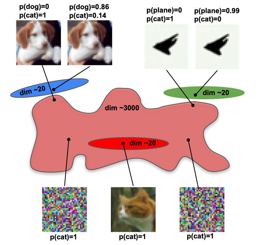
Visualization of our main argument: We show that a network’s perceptual manifold (PM) for any class concept (e.g. cat), defined to be the set of all images confidently perceived by the network as that class, is extremely high dimensional: 3060 out of a total of 3072 for CIFAR10 (large red manifold) and ≈135,000 out of 150,528 for CLIP and ImageNet. In contrast natural images perceived by humans as any class (e.g. dogs, airplanes or cats (blue, green and bright red manifolds)) are only ≈20 dimensional. This indicates that machine and human PMs for any concept are exponentially misaligned: there are exponentially many inputs confidently perceived as any given concept by machines, but not by humans (e.g. the two noise images in the network’s cat perceptual manifold). This exponential misalignment also explains the origin of adversarial examples: e.g. because the network’s cat PM fills up so much of image space, any other input (e.g. dog or airplane) is extremely close to it.
So the core idea is that adversarial examples are absurdly plentiful relative to good images, and this is where the “exponential misalignment” comes from. Similar to how you change the volume of a cube exponentially as you put on more dimensions, the difference in volume between human and machine PMs grows exponentially with the difference in dimensionality.
There are subtleties that are important here that are key for actually verifying the hypothesis. There are ways that you can increase dimension without changing volume, for instance. In fact, they are implicitly using dimensionality as a faithful volume measure in this entire paper, and there are a host of issues that come from this.
You can have adversarial examples make a very high dimensional set, have them be close to every other image in the space, and have that set have very small volume. You could have thin tubes cover the space, you could have a high-dimensional dust cloud, you could have a lot of things that do this and they could explain the observation of adversarial examples being near everything without needing them to take up a lot of volume. I’d personally guess that they do actually have a lot of volume, but they didn’t check this directly, and the volume probably doesn’t scale as dramatically as the dimensionality estimates.
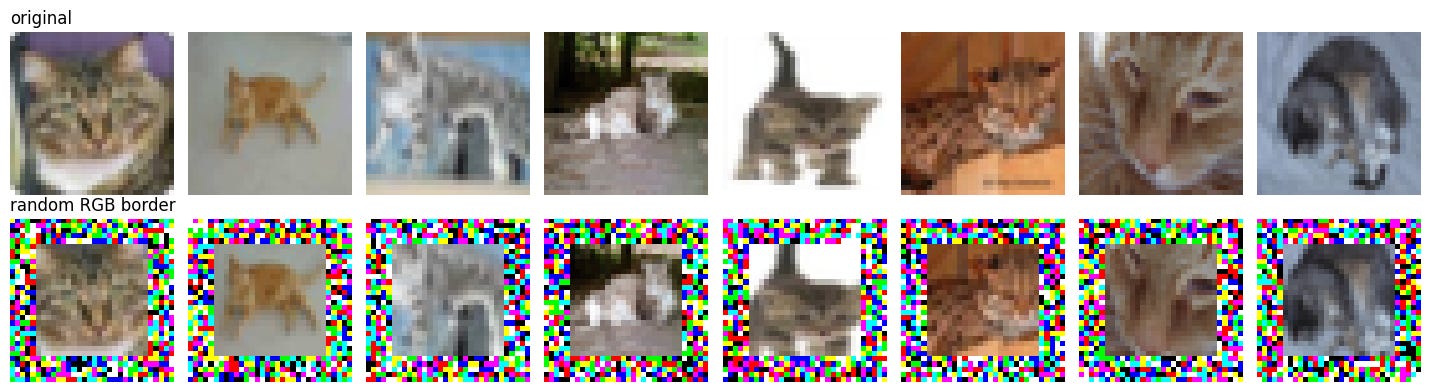
Another problem in this section is the conflation of the dimensionality of natural images and that of the human PM. This tilts the conclusion unfairly; the human PM is much much higher dimensional than their calculations, you can see this trivially by imagining a teeny tiny bit of noise covering the image. You’d still classify all of these images as a cat or whatever, and now the human PM is technically of maximally high dimension! The 2-nearest-neighbors (2NN) method of dimensionality estimation they use is particularly sensitive to this because it’s a local measure, but the participation ratio (PR) is not. For this, you can surround your image or object of interest with high-amplitude noise. PR will call this high-dimensional, and you will still see a cat. With very little effort, I got both estimators to reliably class the human PM as roughly ~250 dimensional.
The other issue is in estimating the dimensionality of the machine PM. It turns out both estimators are extremely sensitive to how you construct examples! What the authors did was initialize at noise, then gradient ascent into the PM of the model. When looking at a bunch of adversarial examples that came from this, dimensionality estimates are nearly the whole available dimensionality! Wild stuff. Turns out, if you initialize at a uniform color, dimensionality estimates are much smaller. I managed to get ~3 dimensional for the PR estimate and ~13 from 2NN with this method.
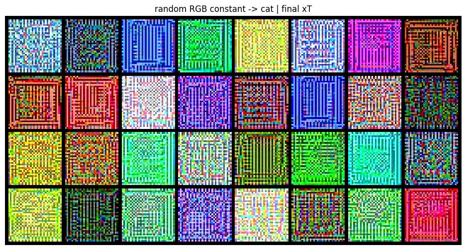
This obviously isn’t correct, in part because the typical meaning of dimensionality kind of breaks down out here, but it goes to show that these methods are extremely sensitive to how you use them! The authors of this paper did not justify these choices, they just made them in the background. It just so happens to be that they chose the way of estimating machine PM dimensionality that would give the largest values, and the way of estimating human PM that would give very low ones.
In all fairness, initializing at noise is reasonable most of the time, and naively estimating the dimensionality of natural images like this makes sense, but it seriously does not work for demonstrating the hypothesis of this paper. As a result I’m suspicious of the authors, but not that suspicious. I’m pretty optimistic about this type of hypothesis and exploration, but it must be done more rigorously in order to get anywhere. It’s very easy to get lost in high-dimensional space.
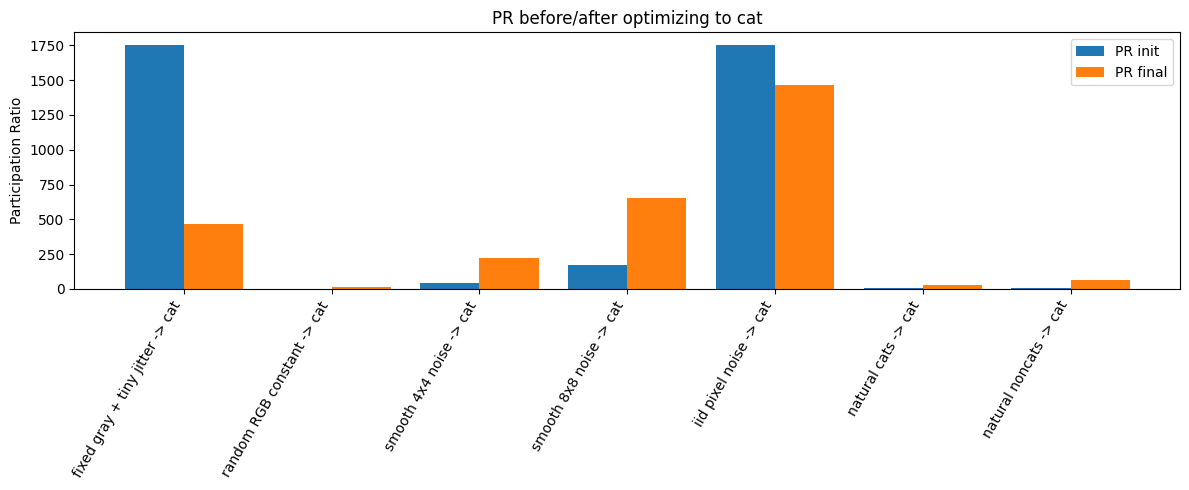
You’ve reached the end of the post! Here are some other outputs. These methods of dim estimation are pretty cool, but they are super sensitive to how you do it and the structure of your data.
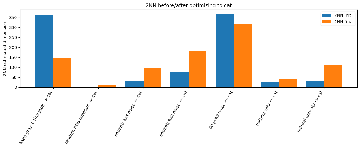
https://github.com/sanskriti-ss/exponential_extension
The files used for the above are PRestimatebreak and noisydimsanitycheck.
Perhaps in the future I will compile all this more cleanly and clearly and rewrite this post and the code. Certainly if the paper ever becomes a problem (popular) I will. Plausibly I will in the meantime anyway, it’s a nice piece to have, this iteration is more of an early “hey this is fucked up” than a serious attempt at getting it retracted or fixed.